Making Sense of Multimodal Models with Partial Information Decomposition

Most multimodal work follows a familiar recipe. Take a vision encoder, bolt on a language model or another sensor, add some cross‑attention, and see whether the validation number goes up. If it does, the second modality is declared “helpful.” If not, people tweak the architecture and move on.

That loop is fine if all you care about is the scoreboard. It is not great if you are trying to understand why a second modality helps or when it is just adding complexity.

The question that pushed me to look at Partial Information Decomposition (PID) is simple:

If adding a new modality improves performance, is it because it carries genuinely new information, because it backs up the first modality, or because the magic only shows up when you combine them?

The NeurIPS 2023 paper Quantifying & Modeling Multimodal Interactions: An Information Decomposition Framework gave me a concrete way to reason about that. It takes the information that two inputs carry about a label and breaks it into four parts instead of one. Even better, the authors show how to estimate those four parts at scale on real multimodal datasets and models.

This post is my attempt to translate that framework into the mental models I actually use when thinking about robots and multimodal systems, and to show where I think it becomes genuinely useful.

How I think about redundancy, uniqueness, and synergy

The formal setup uses three random variables:

• $X_1$: first modality
• $X_2$: second modality
• $Y$: label or target

In my head, I usually instantiate them as:

• $X_1$ – a camera
• $X_2$ – some form of state (LiDAR, proprioception, audio, text)
• $Y$ – “what the system should do next,” a class label, or a scalar target

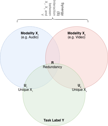
Classical information theory gives you mutual information $I(X_1,X_2;Y)$: the number of bits of uncertainty about $Y$ that disappear when you know both inputs. That is one number. PID says that number is actually the sum of four distinct pieces:

• $R$ is redundancy
• $U_1$ is uniqueness of $X_1$
• $U_2$ is uniqueness of $X_2$
• $S$ is synergy

All four quantities are defined so they are non‑negative and measured in bits, so they share the same units as mutual information.

The way I remember them is as a three‑person team trying to answer a question.

• Redundancy is when both teammates know the same fact about the label. If either shows up to the meeting, you still get that piece of evidence.
• Uniqueness is when only one teammate knows something. Maybe the camera sees the color of an object and the LiDAR does not. That color lives in $U_1$.
• Synergy is when neither teammate can answer alone, but the answer clicks when they compare notes.

A classic synergy example, which the paper also emphasizes, is sarcasm. The text alone reads positive. The tone alone is neutral. The combination tells you the real sentiment is negative.

In robotics I think about a glass door in bright sunlight. The camera sees reflections and a handle. The depth sensor may report free space where the glass panel is. Neither sensor by itself has an obvious “trust me” signal. The safe action comes from spotting that the two views don’t quite agree and reasoning about what that implies. That is synergy in the wild.

PID is useful because it turns those intuitive stories into numbers. Instead of vaguely saying “this is a synergy‑heavy task,” you can look at the estimated $R, U_1, U_2, S$ and see how much of the total information falls into each bucket.

A concrete scenario: hallway robot with camera and LiDAR

To make this less abstract, imagine a simple navigation robot in an office:

• $X_1$: a front‑facing RGB camera
• $X_2$: a 2D LiDAR scan
• $Y$: a discrete “next action” (go forward, turn left, turn right, stop)

Now walk that robot through different situations.

In a wide, empty corridor with good lighting, my intuition is that redundancy $R$ should be high. Either the camera or the LiDAR alone can keep the robot away from walls and obstacles. The camera sees corridor lines, doors, and texture boundaries. LiDAR returns clean, long wall segments. I would expect a large $R$, moderate $U_1$ and $U_2$, and tiny synergy $S$.

In a cluttered storage room, vision has a harder time inferring free space because everything looks messy. LiDAR still sees geometry clearly. Here I expect $U_2$ to climb. The LiDAR brings unique information about safe trajectories that the camera struggles to extract.

Now consider a glass wall or partially open glass door. LiDAR happily fires through the glass and reports free space. The camera sees reflections, frames, maybe people behind the glass. The right behavior is “do not drive straight ahead,” but that judgment does not live in either modality alone. It comes from their mismatch. This is where I expect synergy to spike.

PID gives a way to test those expectations. Gather a dataset of $(x_1,x_2,y)$, run a PID estimator, and see whether $S$ really grows in the tricky edge cases and whether $R$ dominates in simple corridors. The paper does a similar sanity check with synthetic Gaussian mixtures and coordinate transforms, showing that redundancy, uniqueness, and synergy move in ways that match geometric intuition.

How the paper actually computes PID

The nice thing about PID as a concept is that it lets you talk cleanly about interactions. The annoying thing is that computing those four numbers is not trivial once $X_1$ and $X_2$ become high‑dimensional or continuous.

Liang and collaborators borrow a particular PID definition from Bertschinger and colleagues that expresses redundancy, uniqueness, and synergy as solutions to optimization problems over a family of joint distributions that match the observed pairwise statistics $p(x_1,y)$ and $p(x_2,y)$ but relax the coupling between the two modalities. That definition has good theoretical properties, but the optimization over distributions is only manageable in small discrete cases.

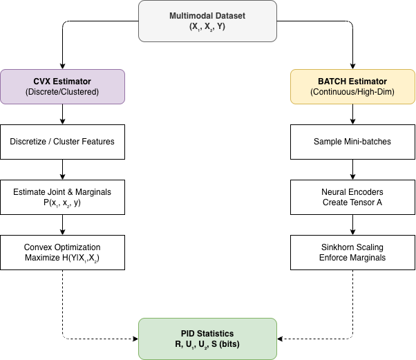
The paper’s main technical contribution is two estimators that scale:

• CVX, a convex optimization method for discretized features
• BATCH, a neural, batch‑based method for continuous and high‑dimensional data

The way I remember them is:

• CVX is “PID over histograms.”
• BATCH is “PID as a small trainable joint model on mini‑batches.”

CVX in my mental model

CVX assumes features and labels can be discretized or clustered into a manageable number of states per variable. Think of clustering image embeddings into a few dozen visual tokens, doing the same for text or other inputs, and keeping labels as finite classes. That gives you an empirical joint distribution $p(x_1,x_2,y)$ and marginals $p(x_1,y)$, $p(x_2,y)$.

From there, CVX looks at all distributions $q(x_1,x_2,y)$ that match those marginals and chooses the one that maximizes the conditional entropy $H_q(Y | X_1,X_2)$. That maximum‑entropy distribution reflects “the least committed coupling between the two modalities that still agrees with what we actually see at the single‑modality level.” The authors show that exactly this optimization recovers the redundancy and uniqueness terms in the Bertschinger PID.

To me, that translates to:

CVX takes your discretized dataset, finds the most agnostic joint coupling consistent with the observed label–modality relationships, and from that coupling you can read off redundancy, uniqueness, and synergy.

It is exact for the discretized distribution and works well for small synthetic examples and some real tasks where clustering makes sense.

BATCH in my mental model

BATCH exists for everything that does not fit in tidy histograms: continuous features, high‑dimensional embeddings, raw sensor logs.

It works on mini‑batches. For a batch of $m$ examples, it:

1. Passes $X_1$ and $X_2$ through separate encoders to get embeddings.
2. Builds a three‑dimensional tensor $A \in \mathbb{R}^{m \times m \times |Y|}$, where each entry $A[i,j,y]$ is an exponentiated similarity between the representation of $x_1^{(i)}$ and $x_2^{(j)}$ given label $y$.
3. Uses approximations to $p(y \mid x_1)$ and $p(y \mid x_2)$, learned by unimodal classifiers, and a differentiable Sinkhorn–Knopp scaling procedure to adjust $A$ so that its marginals line up with those conditionals. The result is a normalized joint distribution $\tilde{q}$ over the batch that lies in the same marginal family $\Delta_p$.
4. Computes a trivariate mutual information $I_{\tilde{q}}(X_1;X_2;Y)$ from $\tilde{q}$ and maximizes it with respect to the encoder parameters over many mini‑batches.

The simplified picture in my head is:

BATCH is a small neural module that, for each batch, learns a joint distribution over the two modalities and the label that agrees with what your unimodal classifiers think, and that tries to make the mutual information between modalities and label as informative as possible. Once that module converges, you treat its learned distribution as your joint and run the same PID formulas on it.

Between CVX and BATCH, you cover both discretized and continuous regimes. The authors have released code that wraps all of this, so you do not have to rebuild it from scratch.

What their experiments convinced me of

Once the estimators are in place, the paper asks three main questions:

1. Do these estimators behave properly on cases where we know the answer
2. What do real multimodal datasets look like under this lens
3. What kinds of interactions are current models actually learning

On synthetic data, both CVX and BATCH recover the exact PID values for simple logic functions (AND, OR, XOR) and behave sensibly on higher‑dimensional generative setups where labels depend on different mixes of shared and unique latent factors. That is a basic but important sanity check.

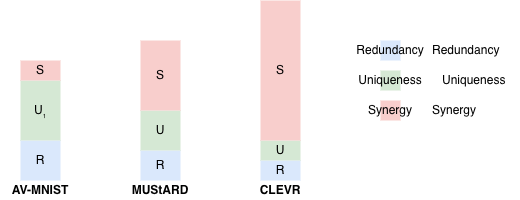
On real data, a few patterns match intuition nicely. On AV‑MNIST and some medical datasets, one modality carries much more unique information than the other and synergy is relatively small, consistent with strong unimodal baselines. On sarcasm and humor datasets such as UR‑FUNNY and MUStARD, synergy is significantly higher, reflecting the need to combine language with audio or visual cues. On VQA 2.0 and CLEVR, synergy is especially large, which lines up with how those benchmarks are constructed so that neither the question text nor the image alone is sufficient.

The authors also collect human judgments of redundancy, uniqueness, and synergy for sampled datapoints. After rescaling the human ratings to the same total magnitude as the PID estimates, the dominant interaction type picked by humans matches the PID values on several datasets, with decent inter‑annotator agreement. That reassures me that these numbers are not just artifacts of an arbitrary definition.

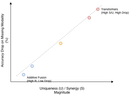
For model analysis, the results are both unsurprising and sobering. Across a range of fusion architectures, redundancy is consistently the easiest interaction type to capture, uniqueness is harder, and synergy is hardest. Additive and agreement‑based methods shine on redundancy‑heavy tasks, while tensor fusion and transformer‑style models do better on synergy‑heavy datasets.

The part that changed how I think about sensor importance was the robustness experiment. When they remove one modality at test time and look at the drop in performance, it correlates strongly with that modality’s uniqueness $U_i$. In regimes where uniqueness is very small, synergy $S$ becomes the relevant predictor: even if neither modality has much unique information, if the task relies on their interaction, removing one of them still hurts. Redundancy, as you would hope, does not correlate with large drops.

In other words, PID can tell you which sensors are “optional” and which are “sacred” before you start ripping cables out.

How I’d use PID in practice

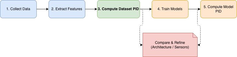
For me, PID is most valuable as an analysis layer around the usual training loop. If I were starting a new multimodal project today, I would use it in three places.

1. Before heavy modeling: quantify the dataset

Given a new pair of modalities and labels, I would first extract features and run dataset‑level PID on $(X_1,X_2,Y)$. If redundancy is huge and synergy is negligible, and one modality has most of the uniqueness, that tells me a lot:

• a fancy cross‑attention fusion block is probably overkill
• I should focus on the stronger modality and keep the other mostly for robustness and interpretability

If synergy is substantial, especially on the edge cases I care about, that justifies investing in more expressive interaction mechanisms such as tensor fusion, cross‑attention, or multimodal transformers.

2. After training: check what models actually use

Once I have trained a few candidate models, I can run PID on $(X_1,X_2,\hat{Y})$ to see what each model relies on.

If the dataset itself looks synergy‑heavy but a particular model’s predictions show almost no synergy, even if its top‑line accuracy is decent, I know it is probably exploiting some shortcut and will break on distribution shift. If another model tracks the dataset’s redundancy/uniqueness/synergy profile more closely, that is a good sign that its inductive bias matches the task.

3. Thinking about robustness in a structured way

Instead of treating sensor ablations as ad‑hoc tests, I can use $U_1, U_2, S$ as a guide. High uniqueness or strong synergy for a modality means its failure is a real risk, and I should prioritize fallback strategies, monitoring, or redundancy there. If a modality is mostly redundant, its loss should hurt less, and if it does not, that is an interesting debugging signal.

In short, PID does not replace accuracy, ROC curves, or any of the usual metrics. What it offers is a way to answer the question that got me interested in the first place:

For this task and this model, what is the second modality actually doing for me—adding new information, backing up the first modality, or enabling interactions that neither can handle alone?

Why this was worth the deep dive

There are many ways to talk about multimodal learning: contrastive objectives, co‑training, redundancy reduction, representation alignment. PID gives something slightly different. It gives a four‑way breakdown of task‑relevant information that:

• has a clean information‑theoretic foundation
• is directly interpretable in bits
• and can now be estimated on real multimodal datasets and models

For me, that is enough to keep it around. When the next shiny multimodal architecture drops, I still want to know: is it mainly boosting redundancy, tapping into previously unused uniqueness, or finally capturing the synergy the task always demanded. PID is one of the few tools that lets me ask that question in a way that has both numbers and intuition behind it.

References

• P. P. Liang et al., “Quantifying & Modeling Multimodal Interactions: An Information Decomposition Framework,” NeurIPS 2023.
• PID code and trained models repository
• Paper on arXiv
• NeurIPS proceedings